(Sample) Transfer Function Analysis and Design Tool - Result -
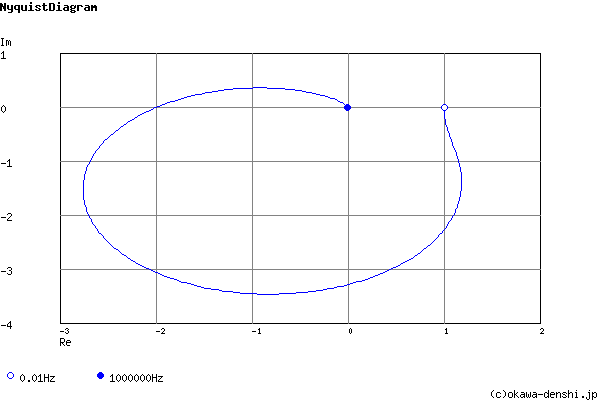
Calculated the Transfer Function, displayed on graphs, showing Bode diagram, Nyquist diagram, Impulse response and Step response.
Transfer Function Analysis
(Sample) Transfer Function:
| G(s)= |
s+10000 s3+30s2+500s+10000 |
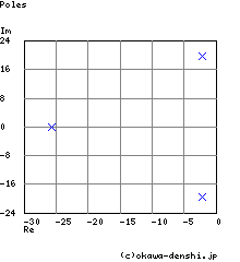
Pole(s)
p = -2.1552679847381 +19.611717445798i
|p|= 3.1400937168562[Hz]
p = -25.689464030524
|p|= 4.0886051858393[Hz]
p = -2.1552679847381-19.611717445798i
|p|= 3.1400937168562[Hz]
|p|= 3.1400937168562[Hz]
p = -25.689464030524
|p|= 4.0886051858393[Hz]
p = -2.1552679847381-19.611717445798i
|p|= 3.1400937168562[Hz]
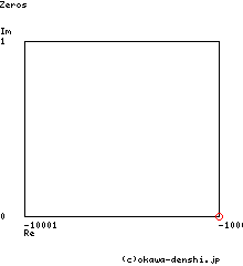
Zero(s)
z = -10000
|z|= 1591.549430919[Hz]
|z|= 1591.549430919[Hz]
Phase margin
pm= -21[deg] (f =4[Hz])
Oscillation frequency:
f = 3.1213017740203[Hz]
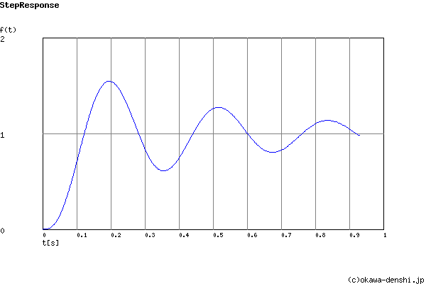
Overshoot (in absolute value)
The 1st peak gpk = 1.55 (t =0.2[sec])
The 2nd peak gpk = 0.61 (t =0.36[sec])
The 3rd peak gpk = 1.28 (t =0.52[sec])
The 2nd peak gpk = 0.61 (t =0.36[sec])
The 3rd peak gpk = 1.28 (t =0.52[sec])
Final value of the step response (on the condition that the system converged when t goes to infinity)
g(∞) = 1
Frequency analysis
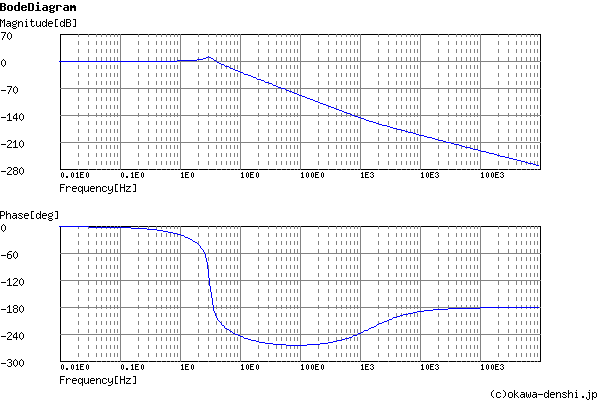
Gain characteristics at the Bode Diagram (provides up to 1 minute)
Phase characteristics at the Bode Diagram (provides up to 1 minute)
Bode Diagram text data (provides up to 1 minute)
Transient analysis